what approximations did you have to make to predict the electron currents?

Magnets exert forces and torques on each other due to the rules of electromagnetism. The forces of allure field of magnets are due to microscopic currents of electrically charged electrons orbiting nuclei and the intrinsic magnetism of primal particles (such as electrons) that make upwards the fabric. Both of these are modeled quite well as tiny loops of current called magnetic dipoles that produce their own magnetic field and are affected by external magnetic fields. The most uncomplicated force between magnets is the magnetic dipole–dipole interaction. If all of the magnetic dipoles that make up two magnets are known then the internet force on both magnets can exist determined past summing upwards all these interactions betwixt the dipoles of the first magnet and that of the second.

Information technology is ofttimes more convenient to model the force between two magnets equally being due to forces between magnetic poles having magnetic charges spread over them. Positive and negative magnetic charge is always connected by a string of magnetized material; isolated magnetic charge does non exist. This model works well in predicting the forces between simple magnets where good models of how the magnetic charge is distributed are available.

Magnetic poles vs. diminutive currents [edit]

Magnetic-charge model for H and Ampère's model for B yield the identical field outside of a magnet. Inside they are very unlike.

The field of a magnet is the sum of fields from all magnetized volume elements, which consist of modest magnetic dipoles on an atomic level. The straight summation of all those dipole fields would require three-dimensional integration just to obtain the field of one magnet, which may be intricate.

In case of a homogeneous magnetization, the trouble can exist simplified at least in two unlike ways, using Stokes' theorem. Upon integration along the direction of magnetization, all dipoles forth the line of integration abolish each other, except at the magnet's end surface. The field then emerges but from those (mathematical) magnetic charges spread over the magnet'due south end facets. On the contrary, when integrating over a magnetized area orthogonal to the direction of magnetization, the dipoles within this area cancel each other, except at the magnet'due south outer surface, where they (mathematically) sum up to a ring current. This is chosen Ampère model. In both models, only two-dimensional distributions over the magnet's surface have to exist considered, which is simpler than the original three-dimensional problem.

Magnetic-charge model: In the magnetic-accuse model, the pole surfaces of a permanent magnet are imagined to be covered with so-chosen magnetic charge, north pole particles on the n pole and due south pole particles' on the southward pole, that are the source of the magnetic field lines. The field due to magnetic charges is obtained through Coulomb'due south law with magnetic instead of electric charges. If the magnetic pole distribution is known, and so the pole model gives the verbal distribution of the magnetic field intensity H both inside and outside the magnet. The surface charge distribution is compatible, if the magnet is homogeneously magnetized and has flat end facets (such as a cylinder or prism).

Ampère model: In the Ampère model, all magnetization is due to the consequence of microscopic, or atomic, circular jump currents, also chosen Ampèrian currents throughout the material. The cyberspace effect of these microscopic bound currents is to make the magnet behave as if there is a macroscopic electrical electric current flowing in loops in the magnet with the magnetic field normal to the loops. The field due to such currents is then obtained through the Biot–Savart law. The Ampère model gives the correct magnetic flux density B both within and outside the magnet. It is sometimes difficult to calculate the Ampèrian currents on the surface of a magnet.

Magnetic dipole moment [edit]

Far abroad from a magnet, its magnetic field is virtually always described (to a adept approximation) by a dipole field characterized past its total magnetic dipole moment, m . This is true regardless of the shape of the magnet, and then long as the magnetic moment is not-aught. One characteristic of a dipole field is that the strength of the field falls off inversely with the cube of the distance from the magnet's center.

The magnetic moment of a magnet is therefore a measure out of its forcefulness and orientation. A loop of electric current, a bar magnet, an electron, a molecule, and a planet all have magnetic moments. More precisely, the term magnetic moment normally refers to a system's magnetic dipole moment, which produces the first term in the multipole expansion^{[notation ane]} of a general magnetic field.

Both the torque and strength exerted on a magnet past an external magnetic field are proportional to that magnet'south magnetic moment. The magnetic moment is a vector: information technology has both a magnitude and management. The management of the magnetic moment points from the south to north pole of a magnet (inside the magnet). For example, the direction of the magnetic moment of a bar magnet, such as the one in a compass is the management that the n poles points toward.

In the physically right Ampère model, magnetic dipole moments are due to infinitesimally pocket-size loops of electric current. For a sufficiently small loop of current, I, and area, A , the magnetic dipole moment is:

$${\displaystyle \mathbf {1000} =I\mathbf {A} ,}$$

where the direction of chiliad is normal to the surface area in a management determined using the electric current and the right-hand rule. Equally such, the SI unit of magnetic dipole moment is ampere meterⁱⁱ. More precisely, to business relationship for solenoids with many turns the unit of magnetic dipole moment is Ampere-turn meter^two.

In the magnetic-accuse model, the magnetic dipole moment is due to ii equal and opposite magnetic charges that are separated by a distance, d. In this model, m is similar to the electrical dipole moment p due to electrical charges:

$${\displaystyle g=q_{\mathrm {chiliad} }d,}$$

where q _m is the 'magnetic charge'. The management of the magnetic dipole moment points from the negative south pole to the positive n pole of this tiny magnet.

Magnetic force due to non-uniform magnetic field [edit]

Top: ${\displaystyle \mathbf {B} }$ , the force on magnetic north-poles.
Bottom: ${\displaystyle \mathbf {\nabla } |\mathbf {B} |}$ , the strength on aligned dipoles, such as iron particles.

Magnets are fatigued along the magnetic field slope. The simplest case of this is the attraction of opposite poles of two magnets. Every magnet produces a magnetic field that is stronger near its poles. If opposite poles of two separate magnets are facing each other, each of the magnets are drawn into the stronger magnetic field well-nigh the pole of the other. If like poles are facing each other though, they are repulsed from the larger magnetic field.

The magnetic-charge model predicts a correct mathematical form for this forcefulness and is easier to sympathise qualitatively. For if a magnet is placed in a uniform magnetic field then both poles will feel the same magnetic force but in opposite directions, since they accept opposite magnetic charge. But, when a magnet is placed in the non-compatible field, such equally that due to another magnet, the pole experiencing the large magnetic field will experience the large force and in that location will exist a net force on the magnet. If the magnet is aligned with the magnetic field, corresponding to ii magnets oriented in the aforementioned direction near the poles, and so it volition exist drawn into the larger magnetic field. If it is oppositely aligned, such as the case of ii magnets with like poles facing each other, then the magnet will exist repelled from the region of higher magnetic field.

In the Ampère model, there is also a force on a magnetic dipole due to a not-compatible magnetic field, but this is due to Lorentz forces on the current loop that makes up the magnetic dipole. The force obtained in the case of a current loop model is

$${\displaystyle \mathbf {F} =\nabla \left(\mathbf {one thousand} \cdot \mathbf {B} \right),}$$

where the slope ∇ is the change of the quantity k · B per unit of measurement distance, and the direction is that of maximum increase of m · B . To sympathise this equation, annotation that the dot product m · B = mB cos(θ), where m and B represent the magnitude of the m and B vectors and θ is the angle between them. If g is in the same direction as B so the dot product is positive and the slope points 'uphill' pulling the magnet into regions of higher B-field (more than strictly larger m ·B). B represents the strength and direction of the magnetic field. This equation is strictly only valid for magnets of zero size, but is oft a good approximation for not likewise large magnets. The magnetic forcefulness on larger magnets is adamant past dividing them into smaller regions having their own m then summing upward the forces on each of these regions.

Magnetic-charge model [edit]

The magnetic-charge model assumes that the magnetic forces between magnets are due to magnetic charges near the poles. This model works even close to the magnet when the magnetic field becomes more complicated, and more than dependent on the detailed shape and magnetization of the magnet than just the magnetic dipole contribution. Formally, the field can be expressed as a multipole expansion: A dipole field, plus a quadrupole field, plus an octopole field, etc. in the Ampère model, but this can be very cumbersome mathematically.

Calculating the magnetic force [edit]

Calculating the attractive or repulsive force between two magnets is, in the general case, a very complex operation, equally it depends on the shape, magnetization, orientation and separation of the magnets. The magnetic-accuse model does depend on some knowledge of how the 'magnetic charge' is distributed over the magnetic poles. It is simply truly useful for simple configurations fifty-fifty then. Fortunately, this restriction covers many useful cases.

Force between ii magnetic poles [edit]

If both poles are pocket-sized enough to exist represented as single points and so they tin can be considered to be point magnetic charges. Classically, the force between 2 magnetic poles is given by:^[1]

$${\displaystyle F={{\mu q_{m1}q_{m2}} \over {4\pi r^{two}}}}$$

where

• F is force (SI unit: newton)
• q _chiliadi and q _m2 are the magnitudes of magnetic accuse on magnetic poles (SI unit: ampere-meter)
• μ is the permeability of the intervening medium (SI unit: tesla meter per ampere, henry per meter or newton per ampere squared)
• r is the separation (SI unit: meter).

The pole description is useful to practicing magneticians who design existent-world magnets, but real magnets have a pole distribution more circuitous than a single north and due south. Therefore, implementation of the pole idea is not elementary. In some cases, one of the more complex formulas given below volition exist more useful.

Forcefulness between two nearby magnetized surfaces of area A [edit]

The mechanical force between 2 nearby magnetized surfaces tin can be calculated with the following equation. The equation is valid just for cases in which the effect of fringing is negligible and the volume of the air gap is much smaller than that of the magnetized material, the force for each magnetized surface is:^{[2] [three] [4]}

$${\displaystyle F={\frac {\mu _{0}H^{2}A}{ii}}={\frac {B^{2}A}{2\mu _{0}}}}$$

where:

• A is the expanse of each surface, in m^two
• H is their magnetizing field, in A/m.
• μ ₀ is the permeability of infinite, which equals 4π×10⁻⁷ T·1000/A
• B is the flux density, in T

The derivation of this equation is analogous to the force between two nearby electrically charged surfaces,^[5] which assumes that the field in between the plates is uniform.

Force between two bar magnets [edit]

Field of ii alluring cylindrical bar magnets

Field of two repelling cylindrical bar magnets

The force betwixt two identical cylindrical bar magnets placed end to end at great altitude ${\displaystyle ten\gg R}$ is approximately:^[2]

$${\displaystyle F\simeq \left[{\frac {B_{0}^{2}A^{2}\left(L^{2}+R^{2}\right)}{\pi \mu _{0}L^{2}}}\right]\left[{\frac {i}{ten^{two}}}+{\frac {1}{(x+2L)^{two}}}-{\frac {2}{(x+L)^{2}}}\right]}$$

where

• B₀ is the flux density very close to each pole, in T,
• A is the expanse of each pole, in chiliad^two,
• 50 is the length of each magnet, in m,
• R is the radius of each magnet, in chiliad, and
• ten is the separation between the two magnets, in m

$${\displaystyle B_{0}={\frac {\mu _{0}}{2}}Thou}$$

relates the flux density at the pole to the magnetization of the magnet.

Notation that these formulations presume point-like magnetic-charge distributions instead of a uniform distribution over the end facets, which is a skillful approximation only at relatively not bad distances. For intermediate distances, numerical methods must be used.

Forcefulness between two cylindrical magnets [edit]

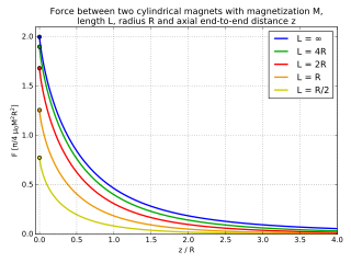
Verbal force between two coaxial cylindrical bar magnets for several aspect ratios.

For two cylindrical magnets with radius ${\displaystyle R}$ , and length ${\displaystyle 50}$ , with their magnetic dipole aligned, the force tin exist computed analytically using elliptic integrals.^[vi] In the limit ${\displaystyle x\gg R}$ , the forcefulness can exist approximated by,^[vii]

$${\displaystyle F(x)\simeq {\frac {\pi \mu _{0}}{4}}M^{2}R^{4}\left[{\frac {one}{10^{2}}}+{\frac {1}{(x+2L)^{2}}}-{\frac {two}{(10+L)^{ii}}}\correct]}$$

Where ${\displaystyle 1000}$ is the magnetization of the magnets and ${\displaystyle x}$ is the distance between them. For small values of ${\displaystyle x}$ , the results are erroneous every bit the force becomes large for close-to-zero distance.

If the magnet is long ( ${\displaystyle L\gg R}$ ), a measurement of the magnetic flux density very shut to the magnet ${\displaystyle B_{0}}$ is roughly related to ${\displaystyle M}$ by the formula

$${\displaystyle B_{0}={\frac {\mu _{0}}{2}}M.}$$

The effective magnetic dipole moment can be written as

$${\displaystyle k=MV}$$

where ${\displaystyle V}$ is the volume of the magnet. For a cylinder this is ${\displaystyle 5=\pi R^{2}50}$ , and ${\displaystyle Thousand}$ is the magnetisation field of the dipole.

When ${\displaystyle 50\ll x}$ the point dipole approximation is obtained,

$${\displaystyle F(ten)={\frac {3\pi \mu _{0}}{two}}Thou^{2}R^{four}L^{2}{\frac {1}{10^{iv}}}={\frac {3\mu _{0}}{2\pi }}Chiliad^{2}5^{2}{\frac {1}{x^{4}}}={\frac {iii\mu _{0}}{ii\pi }}m_{1}m_{ii}{\frac {1}{x^{four}}}}$$

Which matches the expression of the force between 2 magnetic dipoles.

Ampère model [edit]

French scientist André Marie Ampère plant that the magnetism produced by permanent magnets and the magnetism produced by electromagnets are the aforementioned kind of magnetism.

Because of that, the force of a permanent magnet can exist expressed in the same terms as that of an electromagnet.

The strength of magnetism of an electromagnet that is a flat loop of wire through which a current flows, measured at a distance that is corking compared to the size of the loop, is proportional to that current and is proportional to the surface area of that loop.

For purpose of expressing the force of a permanent magnet in same terms every bit that of an electromagnet, a permanent magnet is thought of equally if information technology contains small electric current-loops throughout its volume, and then the magnetic strength of that magnet is constitute to be proportional to the electric current of each loop (in Ampere), and proportional to the surface of each loop (in square meter), and proportional to the density of current-loops in the material (in units per cubic meter), so the dimension of strength of magnetism of a permanent magnet is Ampere times foursquare meter per cubic meter, is Ampere per meter.

That is why Ampere per meter is the correct unit of magnetism, even though these small current loops are not actually nowadays in a permanent magnet.

The validity of Ampere's model means that information technology is allowable to think of the magnetic material every bit if it consists of current-loops, and the total event is the sum of the effect of each electric current-loop, and and so the magnetic effect of a real magnet tin exist computed as the sum of magnetic furnishings of tiny pieces of magnetic textile that are at a distance that is great compared to the size of each piece.

This is very useful for calculating magnetic force-field of a real magnet ; It involves summing a large corporeality of small forces and you should not do that by hand, simply let your figurer practise that for you ; All that the computer program needs to know is the force between modest magnets that are at corking altitude from each other.

In such computations it is often causeless that each (same-size) minor slice of magnetic material has an equally strong magnetism, just this is not always truthful : a magnet that is placed near another magnet can change the magnetization of that other magnet. For permanent magnets this is usually only a small change, but if yous take an electromagnet that consists of a wire wound round an atomic number 26 cadre, and you bring a permanent magnet near to that core, then the magnetization of that core can modify drastically (for example, if there is no current in the wire, the electromagnet would not exist magnetic, but when the permanent magnet is brought near, the core of the electromagnet becomes magnetic).

Thus the Ampere model is suitable for computing the magnetic force-field of a permanent magnet, but for electromagnets it can be ameliorate to utilise a magnetic-circuit approach.

Magnetic dipole–dipole interaction [edit]

If ii or more than magnets are pocket-size enough or sufficiently distant that their shape and size is not of import and so both magnets can be modeled as existence magnetic dipoles having a magnetic moments 1000 ₁ and g _ii. In case of uniformly magnetized spherical magnets this model is precise even at finite size and distance, as the exterior field of such magnets is exactly a dipole field.^[8]

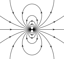
Magnetic field of an platonic dipole.

The magnetic field of a magnetic dipole in vector notation is:

$${\displaystyle \mathbf {B} (\mathbf {m} ,\mathbf {r} )={\frac {\mu _{0}}{4\pi r^{3}}}\left(three(\mathbf {m} \cdot {\hat {\mathbf {r} }}){\chapeau {\mathbf {r} }}-\mathbf {1000} \right)+{\frac {2\mu _{0}}{3}}\mathbf {thou} \delta ^{3}(\mathbf {r} )}$$

where

• B is the field
• r is the vector from the position of the dipole to the position where the field is existence measured
• r is the absolute value of r: the distance from the dipole
• ${\displaystyle {\hat {\mathbf {r} }}=\mathbf {r} /r}$ is the unit vector parallel to r;
• m is the (vector) dipole moment
• μ ₀ is the permeability of free space
• δ ⁱⁱⁱ is the three-dimensional delta function.^{[note ii]}

This is exactly the field of a point dipole, exactly the dipole term in the multipole expansion of an arbitrary field, and approximately the field of any dipole-like configuration at large distances.

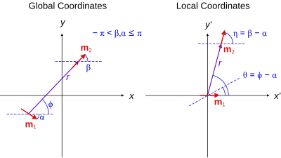
Frames of reference for computing the forces between two dipoles

Forcefulness betwixt coaxial cylinder magnets. Co-ordinate to the dipole approximation, the forcefulness drops proportional to ${\displaystyle 1/z^{4}}$ for large distance z, resulting in slopes of −iv in the log–log plot.

If the coordinate system is shifted to center information technology on m ₁ and rotated such that the z-axis points in the direction of yard ₁ then the previous equation simplifies to^[9]

$${\displaystyle {\begin{aligned}B_{z}(\mathbf {r} )&={\frac {\mu _{0}}{4\pi }}m_{1}\left({\frac {three\cos ^{2}\theta -one}{r^{3}}}\right)\\B_{x}(\mathbf {r} )&={\frac {\mu _{0}}{4\pi }}m_{1}\left({\frac {three\cos \theta \sin \theta }{r^{3}}}\right),\end{aligned}}}$$

where the variables r and θ are measured in a frame of reference with origin in yard _i and oriented such that m ₁ is at the origin pointing in the z-direction. This frame is called Local coordinates and is shown in the Effigy on the right.

The force of one magnetic dipole on another is determined by using the magnetic field of the kickoff dipole given to a higher place and determining the forcefulness due to the magnetic field on the 2d dipole using the force equation given to a higher place. Using vector notation, the force of a magnetic dipole m _one on the magnetic dipole m ₂ is:

$${\displaystyle \mathbf {F} (\mathbf {r} ,\mathbf {m} _{1},\mathbf {m} _{2})={\frac {3\mu _{0}}{4\pi r^{5}}}\left[(\mathbf {m} _{1}\cdot \mathbf {r} )\mathbf {m} _{ii}+(\mathbf {chiliad} _{2}\cdot \mathbf {r} )\mathbf {thou} _{1}+(\mathbf {m} _{1}\cdot \mathbf {m} _{2})\mathbf {r} -{\frac {five(\mathbf {m} _{1}\cdot \mathbf {r} )(\mathbf {g} _{2}\cdot \mathbf {r} )}{r^{2}}}\mathbf {r} \right]}$$

where r is the altitude-vector from dipole moment m ₁ to dipole moment m _ii, with r = || r ||. The force acting on m ₁ is in reverse direction. As an example the magnetic strength for two magnets pointing in the z-direction and aligned on the z-axis and separated by the altitude z is:

${\displaystyle \mathbf {F} (z,m_{ane},m_{ii})=-{\frac {3\mu _{0}m_{1}m_{2}}{two\pi z^{4}}}}$ , z-direction.

The final formulas are shown next. They are expressed in the global coordinate organization,

$${\displaystyle {\begin{aligned}F_{r}(\mathbf {r} ,\alpha ,\beta )&=-{\frac {iii\mu _{0}}{iv\pi }}{\frac {m_{2}m_{i}}{r^{4}}}\left[2\cos(\phi -\alpha )\cos(\phi -\beta )-\sin(\phi -\blastoff )\sin(\phi -\beta )\right]\\F_{\phi }(\mathbf {r} ,\alpha ,\beta )&=-{\frac {3\mu _{0}}{4\pi }}{\frac {m_{2}m_{1}}{r^{iv}}}\sin(two\phi -\blastoff -\beta )\end{aligned}}}$$

Notes [edit]

1. ^ The magnetic dipole portion of the magnetic field can exist understood as being due to one pair of north/south poles. College order terms such as the quadrupole tin can be considered as due to two or more north/south poles ordered such that they accept no lower order contribution. For example the quadrupole configuration has no net dipole moment.
2. ^ δ ³(r) = 0 except at r = (0,0,0), so this term is ignored in multipole expansion.

References [edit]

1. ^ "Basic Relationships". Geophysics.ou.edu. Archived from the original on 2010-07-09. Retrieved 2009-10-nineteen .
2. ^ ^{a b} "Magnetic Fields and Forces". Archived from the original on February 20, 2012. Retrieved 2009-12-24 .
3. ^ "The force produced by a magnetic field". Retrieved 2013-eleven-07 .
4. ^ "Tutorial: Theory and applications of the Maxwell stress tenso" (PDF) . Retrieved 2018-xi-28 .
5. ^ "Force Interim on Capacitor Plates — Collection of Solved Problems". physicstasks.european union . Retrieved 2020-01-20 .
6. ^ Ravaud, R; Lemarquand, K; Babic, Southward; Lemarquand, 5; Akyel, C (2010). "Cylindrical magnets and coils: Fields, forces, and inductances". IEEE Transactions on Magnetics. 46 (nine): 3585–3590. Bibcode:2010ITM....46.3585R. doi:x.1109/TMAG.2010.2049026. S2CID 25586523.
7. ^ Vokoun, David; Beleggia, Marco; Heller, Ludek; Sittner, Petr (2009). "Magnetostatic interactions and forces betwixt cylindrical permanent magnets". Journal of Magnetism and Magnetic Materials. 321 (22): 3758–3763. Bibcode:2009JMMM..321.3758V. doi:10.1016/j.jmmm.2009.07.030.
8. ^ Lehner, Günther (2008). Electromagnetic Field Theory for Engineers and Physicists. p. 309. doi:10.1007/978-iii-540-76306-2. ISBN978-3-540-76305-5.
9. ^ Schill, R. A. (2003). "General relation for the vector magnetic field of a round current loop: A closer look". IEEE Transactions on Magnetics. 39 (2): 961–967. Bibcode:2003ITM....39..961S. doi:10.1109/TMAG.2003.808597.

See also [edit]

• Magnetic motor

adamsfluentsmay.blogspot.com

Source: https://en.wikipedia.org/wiki/Force_between_magnets

Share this post